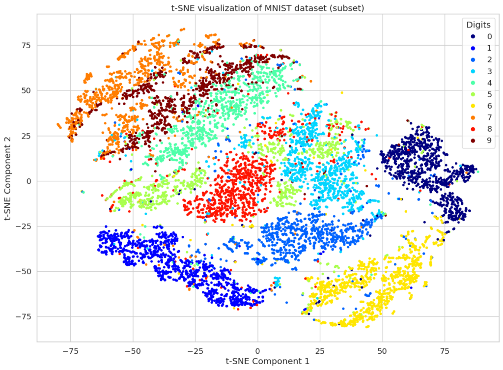
t-SNE in 50 lines of code with PyTorch

t-SNE is one of the most popular dimensional reduction techniques for visualizing high-dimensional data. It preserves the local structure in the high-dimensional dataset – In other words, similar data points that are close to each other should still be close to each other after dimension reduction. One classic example here is applying t-SNE on the MNIST hand-written digits dataset, where we can find nice clusters for each of the digits:

Different digits form different clusters after t-SNE, illustrating that t-SNE successfully preserves the local structure of the original dataset. Figure taken from: t-SNE-Mnist-Dataset

This ToothlessOS Log provides a demo explanation of t-SNE with step by step walk through to help you better understand this beautiful algorithm.

Intuition behind t-SNE

Given a dataset $X$ , t-SNE builds a probability distribution $P$ over pairs of high-dimensional data points. Then, it learns a low dimensional embedding $Y$ by minimizing the KL-divergence between $P$ and a low-dimensional distribution $Q$ . Personally, the keywords that I keep for t-SNE is pairwise distances and matching probability distributions, which we will walk through in the next section. I find it very helpful to use such keywords to capture the objectives of dimensional reduction algorithms – to make sure that I use them properly in practice.

Implementation walkthrough

Step 1: Pairwise squared distances

X_dist = torch.sum((X_mat[:, None, :] - X_mat[None, :, :])**2, axis=-1)

X_dist = torch.sum((X_mat[:, None, :] - X_mat[None, :, :])**2, axis=-1)

We start by computing squared Euclidean distance between all pairs of input points:

d_{ij} = \|x_i – x_j\|^2

Step 2: High dimensional similarities $P(j|i)$

X_sim_scores = torch.exp(-X_dist / (2 * (perplexity ** 2)))
X_cond = X_sim_scores / torch.sum(X_sim_scores, axis=1, keepdim=True)

X_sim_scores = torch.exp(-X_dist / (2 * (perplexity ** 2)))
X_cond = X_sim_scores / torch.sum(X_sim_scores, axis=1, keepdim=True)

The pairwise distances are converted into similarities of each node $i$ with all other nodes $j$ using a Gaussian kernel. We can get the conditional probabilities $P(j|i)$ after normalization:

p_{j|i} = \frac{\exp(-\|x_i – x_j\|^2 / 2\sigma_i^2)}{\sum_{k \neq i} \exp(-\|x_i – x_k\|^2 / 2\sigma_i^2)}

The width of the Gaussian kernel $\sigma_i$ can be tuned via the hyper-parameter perplexity – a smaller $\sigma_i$ means the $\exp(-\|x_i-x_j\|^2 / 2\sigma_i^2)$ term decays very quickly, and the similarity between far away points are almost 0 (i.e. a small number of effective neighbours); while a larger $\sigma_i$ makes the exponential term decays slowly, so far away points gets higher probabilities, resulting in a flatter distribution (i.e. a large number of effective neighbours). In this way, perplexity becomes the most important hyperparameter to tune when using t-SNE.

Warning: for simplicity, this implementation uses a fixed Gaussian bandwidth $\sigma_i$ = perplexity, which is not the same procedure used in original t-SNE. This keeps to code short for now and makes things easier to explain for now. For detailed explanation of perplexity, its tuning, and the original implementation with binary search, please refer to the appendix.

Step 3: Get joint distribution

X_joint = (X_cond + X_cond.T) / (2 * X.shape[0])

X_joint = (X_cond + X_cond.T) / (2 * X.shape[0])

We then symmetrize the conditional probabilities to obtain the joint probabilities $P_{ij}$ :

p_{ij} = \frac{p_{j|i} + p_{i|j}}{2n}

With these three steps, we now have a joint distribution to model the local structure of the high dimensional data points. Now, we will build the low dimensional embeddings and distribution (for similarities) to match this high dimensional distribution.

Step 4: Initialization of low dimensional embeddings Y

Y, _, _, _, _ = PCA(X, n_components=2) # See prereq PCA implementation
Y = torch.tensor(Y, dtype=torch.float32, requires_grad=True)

Y, _, _, _, _ = PCA(X, n_components=2) # See prereq PCA implementation
Y = torch.tensor(Y, dtype=torch.float32, requires_grad=True)

Instead of random initialization, we initialize the low-dimensional embedding with PCA. This usually leads to faster convergence and better results.

Step 5: Low-dimensional similarity/distribution $Q(i, j)$

Y_dist = torch.sum((Y[:, None, :] - Y[None, :, :])**2, axis=-1)
Y_sim_scores = 1 / (1 + Y_dist)
Y_joint = Y_sim_scores / torch.sum(Y_sim_scores)

Y_dist = torch.sum((Y[:, None, :] - Y[None, :, :])**2, axis=-1)
Y_sim_scores = 1 / (1 + Y_dist)
Y_joint = Y_sim_scores / torch.sum(Y_sim_scores)

In the low-dimensional space, we use a Student-t kernel with one degree of freedom to measure similarity:

q_{ij} = \frac{(1 + \|y_i – y_j\|^2)^{-1}}{\sum_{k \neq l} (1 + \|y_k – y_l\|^2)^{-1}}

Why Student-t kernel instead of Gaussian? In the high-dimensional space, t-SNE uses a Gaussian kernel to convert distances into probabilities. The Gaussian kernel decays quickly, which is ideal for capturing local neighborhoods. However, if we used a Gaussian kernel in the low-dimensional space as well, we would run into the crowding problem:

Consider the original dataset lies uniformly on the high dimension sphere with $D = 10$ and radius $2r$ with one data point at the origin. Take the data point at the origin, we consider points that lie between $[0, r)$ to be neighbours and points that lie between $[r, 2r]$ to be far away. The volume of the neighbouring region is $r^D$ while the volume of the far away region is $(2^D-1)r^D$ . In the example here where we reduce D from 10 to 2, we are cramming the 1000x far away data points into only x3 space, causing the crowding. This is part of the paradox that we called the curse of dimensionality. With the Gaussian kernel that decays quickly, we will run into the same issue that we do not have enough space to pack the far away data points into 2D, causing everything to be mixed up.

While the student-t distribution has a heavier tail / decays slowly – it assigns higher similarity to points that are relatively farther apart. This gives more space to the far away data points by allowing them to be placed closer to the center. This help to solve the crowding problem.

Step 6: KL-divergence and optimization

loss = torch.sum(X_joint_clipped * torch.log(X_joint_clipped / Y_joint_clipped))
loss.backward()
optimizer.step()

loss = torch.sum(X_joint_clipped * torch.log(X_joint_clipped / Y_joint_clipped))
loss.backward()
optimizer.step()

We minimize the KL divergence (i.e. matching distributions) between the high dimensional distribution $P$ and the low dimensional distribution $Q$ with respect to the low dimensional embeddings $Y$ . After several iterations of gradient descent, we are able to get the embeddings $Y$ that represents the local structures in the high dimensional dataset, which can be used for visualization.

Full implementation

Limitations and practical notes: This implementation is for demo purpose and not suitable for production: The original t-SNE selects $\sigma_i$ by binary search to match a given perplexity. The code stores full n-by-n matrices, so it does not scale well beyond a few thousand points. Techniques like early exaggeration and momentum are omitted in this demo.

# PCA as a pre-requisite

import numpy as np

def PCA(X: pd.DataFrame, n_components=2):
    # Step 1: Standardize X (& Get covariance matrix) - preprocessing
    X_mat = X.to_numpy()
    X_centered = X_mat - np.mean(X_mat, axis=0, keepdims=True)
    X_std = X_centered / np.std(X_centered, axis=0, keepdims=True)
    X_cov = np.cov(X_std, rowvar=False, ddof=0)

    # Step 2: SVD on X_std
    U, S, Vt = np.linalg.svd(X_std)

    # Step 3: Select n components (e.g., top two) from V and project X onto them
    components = Vt[:n_components, :]
    eigs = S[:n_components]**2

    # Step 4: Project X onto the selected components (Reconstruction)
    X_reduced = X_std @ components.T

    # Step 5: Compute explained variance
    explained_variance = np.sum(eigs) / np.sum(S**2)

    return X_reduced, components, eigs, explained_variance, X_cov

# PCA as a pre-requisite

import numpy as np

def PCA(X: pd.DataFrame, n_components=2):
    # Step 1: Standardize X (& Get covariance matrix) - preprocessing
    X_mat = X.to_numpy()
    X_centered = X_mat - np.mean(X_mat, axis=0, keepdims=True)
    X_std = X_centered / np.std(X_centered, axis=0, keepdims=True)
    X_cov = np.cov(X_std, rowvar=False, ddof=0)

    # Step 2: SVD on X_std
    U, S, Vt = np.linalg.svd(X_std)

    # Step 3: Select n components (e.g., top two) from V and project X onto them
    components = Vt[:n_components, :]
    eigs = S[:n_components]**2

    # Step 4: Project X onto the selected components (Reconstruction)
    X_reduced = X_std @ components.T

    # Step 5: Compute explained variance
    explained_variance = np.sum(eigs) / np.sum(S**2)

    return X_reduced, components, eigs, explained_variance, X_cov

# main t-SNE implementation

import torch
import torch.nn.functional as F

def t_SNE(X: pd.DataFrame, perplexity=30, random_state=42):

    torch.manual_seed(random_state)
    
    # Step 1: Compute Squared Distances
    X_mat = X.to_numpy()
    X_mat = torch.tensor(X_mat, dtype=torch.float32)
    X_dist = torch.sum((X_mat[:, None, :] - X_mat[None, :, :])**2, axis=-1)

    # Step 2: Similarity score & Conditional probabilities (P(j|i))
    X_sim_scores = torch.exp(-X_dist / (2 * (perplexity ** 2))) # Gaussian kernel
    X_sim_scores.fill_diagonal_(0)
    X_cond = X_sim_scores / torch.sum(X_sim_scores, axis=1, keepdim=True) # Normalize

    # Step 3: Symmetrize to get joint probabilities P(i,j)
    X_joint = (X_cond + X_cond.T) / (2 * X.shape[0])
    
    # Step 4: Initialize low-dimensional embedding Y
    # Here, we make use of the PCA function defined earlier
    Y, _, _, _, _ = PCA(X, n_components=2)
    Y = torch.tensor(Y, dtype=torch.float32, requires_grad=True)

    # Step 5: Low dimensional distances => Similarity scores => Joint probabilities Q(i,j)
    Y_dist = torch.sum((Y[:, None, :] - Y[None, :, :])**2, axis=-1)
    Y_sim_scores = 1 / (1 + Y_dist) # Student t-kernel
    Y_sim_scores.fill_diagonal_(0)
    Y_joint = Y_sim_scores / torch.sum(Y_sim_scores)

    # Step 6: Minimize KL Divergence between P and Q using gradient descent
    optimizer = torch.optim.Adam([Y], lr=0.05)
    for epoch in range(1000):
        optimizer.zero_grad()
        # KL(P||Q) = sum(P * log(P/Q))
        Y_joint_clipped = torch.clamp(Y_joint, min=1e-12)
        X_joint_clipped = torch.clamp(X_joint, min=1e-12)
        loss = torch.sum(X_joint_clipped * torch.log(X_joint_clipped / Y_joint_clipped))
        loss.backward()
        optimizer.step()

        if epoch % 100 == 0:
            print(f'Epoch {epoch}, KL Divergence: {loss.item()}')

        # Recompute Q(i,j) for current Y
        Y_dist = torch.sum((Y[:, None, :] - Y[None, :, :])**2, axis=-1)
        Y_sim_scores = 1 / (1 + Y_dist) # Student t-kernel
        Y_sim_scores.fill_diagonal_(0)
        Y_joint = Y_sim_scores / torch.sum(Y_sim_scores)

    return Y.detach().numpy()

# main t-SNE implementation

import torch
import torch.nn.functional as F

def t_SNE(X: pd.DataFrame, perplexity=30, random_state=42):

    torch.manual_seed(random_state)
    
    # Step 1: Compute Squared Distances
    X_mat = X.to_numpy()
    X_mat = torch.tensor(X_mat, dtype=torch.float32)
    X_dist = torch.sum((X_mat[:, None, :] - X_mat[None, :, :])**2, axis=-1)

    # Step 2: Similarity score & Conditional probabilities (P(j|i))
    X_sim_scores = torch.exp(-X_dist / (2 * (perplexity ** 2))) # Gaussian kernel
    X_sim_scores.fill_diagonal_(0)
    X_cond = X_sim_scores / torch.sum(X_sim_scores, axis=1, keepdim=True) # Normalize

    # Step 3: Symmetrize to get joint probabilities P(i,j)
    X_joint = (X_cond + X_cond.T) / (2 * X.shape[0])
    
    # Step 4: Initialize low-dimensional embedding Y
    # Here, we make use of the PCA function defined earlier
    Y, _, _, _, _ = PCA(X, n_components=2)
    Y = torch.tensor(Y, dtype=torch.float32, requires_grad=True)

    # Step 5: Low dimensional distances => Similarity scores => Joint probabilities Q(i,j)
    Y_dist = torch.sum((Y[:, None, :] - Y[None, :, :])**2, axis=-1)
    Y_sim_scores = 1 / (1 + Y_dist) # Student t-kernel
    Y_sim_scores.fill_diagonal_(0)
    Y_joint = Y_sim_scores / torch.sum(Y_sim_scores)

    # Step 6: Minimize KL Divergence between P and Q using gradient descent
    optimizer = torch.optim.Adam([Y], lr=0.05)
    for epoch in range(1000):
        optimizer.zero_grad()
        # KL(P||Q) = sum(P * log(P/Q))
        Y_joint_clipped = torch.clamp(Y_joint, min=1e-12)
        X_joint_clipped = torch.clamp(X_joint, min=1e-12)
        loss = torch.sum(X_joint_clipped * torch.log(X_joint_clipped / Y_joint_clipped))
        loss.backward()
        optimizer.step()

        if epoch % 100 == 0:
            print(f'Epoch {epoch}, KL Divergence: {loss.item()}')

        # Recompute Q(i,j) for current Y
        Y_dist = torch.sum((Y[:, None, :] - Y[None, :, :])**2, axis=-1)
        Y_sim_scores = 1 / (1 + Y_dist) # Student t-kernel
        Y_sim_scores.fill_diagonal_(0)
        Y_joint = Y_sim_scores / torch.sum(Y_sim_scores)

    return Y.detach().numpy()

Appendix: Perplexity

Reference: tsne.pdf

Perplexity is defined as:

\text{Perp}(P_i) = 2^{H(P_i)},\quad H(P_i) = -\sum_{j \neq i} p_{j|i} \log_2 p_{j|i}

,where

P_i = (p_{1|i}, p_{2|i}, \dots, p_{n|i})

is the distribution of “given data point $i$ , the probability of selecting other points as its neighbours”, modelled by the Gaussian kernel of step 2.

Therefore, we have the following chain (Note the monotonicity here):

Smaller $\sigma_i$ (width of Gaussian kernel) => More concentrated distribution => Lower entropy => Lower perplexity
Larger $\sigma_i$ => More flat / even distribution => Higher entropy => Higher perplexity

In this way, we can use binary search to find the $\sigma_i$ for each data point such that its perplexity $P(i)$ matches the value that we set. In this way, perplexity controls the effective number of neighbours for each data point in t-SNE. Usually, we should try multiple perplexity values between 5 and 50 in practice.